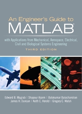
Engineers Guide to MATLAB, An
Pearson (Verlag)
978-0-13-199110-1 (ISBN)
This highly respected guide helps students develop a strong working knowledge of MATLAB that can be used to solve a wide range of engineering problems. Since solving these problems usually involves writing relatively short, one-time-use programs, the authors demonstrate how to effectively develop programs that are compact yet readable, easy to debug, and quick to execute. Emphasis is on using MATLAB to obtain solutions to several classes of engineering problems, so technical material is presented in summary form only.
The new edition has been thoroughly revised and tested for software release 2009.
Dr. Magrab is Emeritus Professor of Mechanical Engineering at the University of Maryland, College Park, Maryland. His research interests include the integration of design and manufacturing, vibrations and acoustics, and the theoretical and experimental analysis of structural systems. Prior to joining the University of Maryland he held supervisory positions in the Center for Manufacturing Engineering, at the National Institute of Standards and Technology (NIST), which included being the head of the Robot Metrology Group and manager of the vertical machining workstation in the Automated Manufacturing Research Facility. He went to NIST after being a professor for almost a decade in the Department of Mechanics at the Catholic University of America in Washington DC. Dr. Magrab is a Life Fellow in the American Society of Mechanical Engineers and a registered professional engineer in Maryland. He has authored seven textbooks and published numerous journal articles. He holds one patent.
List of Examples xiv
Preface to Third Edition xx
1 Introduction 1
Edward B. Magrab
1.1 Introduction 1
1.1.1 Organization of the Book and Its Goals 2
1.1.2 Some Suggestions on How to Use MATLAB 2
1.1.3 Book Notation Conventions 3
1.2 The MATLAB Environment 3
1.2.1 Introduction 3
1.2.2 Preliminaries–Command Window Management 5
1.2.3 Executing Expressions from the MATLAB Command Window–Basic MATLAB Syntax 8
1.2.4 Clarification and Exceptions to MATLAB’S Syntax 11
1.2.5 MATLAB Functions 14
1.2.6 Creating Scripts and Executing Them from the MATLAB Editor 19
1.3 Online Help 29
1.4 The Symbolic Toolbox 33
1.5 Summary of Functions Introduced in Chapter 1 41
Exercises 42
2 Vectors and Matrices 51
Edward B. Magrab
2.1 Introduction 51
2.2 Definitions of Matrices and Vectors 52
2.3 Creation of Vectors 53
2.4 Creation of Matrices 64
2.5 Dot Operations 83
2.6 Mathematical Operations with Matrices 92
2.6.1 Addition and Subtraction 92
2.6.2 Multiplication 92
2.6.3 Determinants 101
2.6.4 Matrix Inverse 104
2.6.5 Solution of a System of Equations 107
2.7 Summary of Functions Introduced in Chapter 2 112
Exercises 113
3 Data Input/Output 127
Edward B. Magrab
3.1 Strings and Annotated Output 127
3.1.1 Creating Strings 127
3.1.2 Converting Numerical Values to Strings and Displaying Them 130
3.2 Entering Data with input 135
3.2.1 Entering a Scalar with input 135
3.2.2 Entering a String with input 136
3.2.3 Entering a Vector with input 137
3.2.4 Entering a Matrix with input 137
3.3 Input/Output Data Files 137
3.4 Cell Arrays 141
3.5 Input Microsoft Excel Files 143
3.6 Summary of Functions Introduced in Chapter 3 144
Exercises 145
4 Program Flow Control 148
Edward B. Magrab
4.1 Introduction—The Logical Operator 148
4.2 Control of Program Flow 151
4.2.1 Branching—If Statement 151
4.2.2 Branching—Switch Statement 154
4.2.3 For Loop 155
4.2.4 While Loop 162
4.2.5 Early Termination of Either a for or a while Loop 166
4.3 Summary of Functions Introduced in Chapter 4 166
Exercises 167
5 Function Creation and Selected MATLAB Functions 172
Edward B. Magrab
5.1 Introduction 173
5.1.1 Why Use Functions 173
5.1.2 Naming Functions 174
5.1.3 Length of Functions 174
5.1.4 Debugging Functions 174
5.2 User-Defined Functions 175
5.2.1 Introduction 175
5.2.2 Function File 175
5.2.3 Subfunctions 181
5.2.4 Anonymous Functions 183
5.2.5 inline 184
5.2.6 Comparison of the Usage of Subfunctions, Anonymous Functions, and inline 185
5.3 User-Defined Functions, Function Handles, and feval 186
5.4 MATLAB Functions that Operate on Arrays of Data 187
5.4.1 Introduction 187
5.4.2 Fitting Data with Polynomials–polyfit/polyval 188
5.4.3 Fitting Data with spline 190
5.4.4 Interpolation of Data–interp1 192
5.4.5 Numerical Integration–trapz 193
5.4.6 Area of a Polygon–polyarea 195
5.4.7 Digital Signal Processing–fft and ifft 196
5.5 MATLAB Functions that Require User-Defined Functions 201
5.5.1 Zeros of Functions–fzero and roots/poly 202
5.5.2 Numerical Integration–quadl and dblquad 207
5.5.3 Numerical Solutions of Ordinary Differential Equations–ode45 212
5.5.4 Numerical Solutions of Ordinary Differential Equations–bvp4c 217
5.5.5 Numerical Solutions of Delay Differential Equations–dde23 231
5.5.6 Numerical Solutions of One-Dimensional Parabolic—Elliptic Partial Differential Equations–pdepe 233
5.5.7 Local Minimum of a Function–fminbnd 235
5.5.8 Numerical Solutions of Nonlinear Equations–fsolve 238
5.6 Symbolic Solutions and Converting Symbolic Expressions into Functions 240
5.7 Summary of Functions Introduced in Chapter 5 246
Exercises 247
6 2D Graphics 265
Edward B. Magrab
6.1 Introduction: Graphics Management 266
6.2 Basic 2D Plotting Commands 269
6.2.1 Introduction 269
6.2.2 Changing a Graph’s Overall Appearance 281
6.2.3 Special Purpose Graphs 281
6.2.4 Reading, Displaying, and Manipulating Digital Images 288
6.3 Graph Annotation and Enhancement 290
6.3.1 Introduction 290
6.3.2 Axes and Curve Labels, Figure Titles, Legends, and Text Placement 290
6.3.3 Filling Regions 294
6.3.4 Greek Letters, Mathematical Symbols, Subscripts, and Superscripts 297
6.3.5 Altering the Attributes of Axes, Curves,Text, and Legends 300
6.3.6 Positioning One Figure Inside Another Figure 304
6.3.7 Interactive Plotting Tools 306
6.3.8 Animation 307
6.4 Examples 310
6.5 Summary of Functions Introduced in Chapter 6 319
Exercises 320
7 3D Graphics 338
Edward B. Magrab
7.1 Lines in 3D 338
7.2 Surfaces 341
7.3 Summary of Functions Introduced in Chapter 7 369
Exercises 370
8 Engineering Statistics 377
Edward B. Magrab
8.1 Descriptive Statistical Quantities 377
8.2 Probability Distributions 383
8.2.1 Discrete Distributions 383
8.2.2 Continuous Distributions 387
8.3 Confidence Intervals 397
8.4 Hypothesis Testing 401
8.5 Linear Regression 404
8.5.1 Simple Linear Regression 404
8.5.2 Multiple Linear Regression 408
8.6 Design of Experiments 415
8.6.1 Single-Factor Experiments: Analysis of Variance 415
8.6.2 Multiple-Factor Factorial Experiments 419
8.7 Summary of Functions Introduced in Chapter 8 435
Exercises 436
9 Dynamics and Vibrations 445
Balakumar Balachandran
9.1 Dynamics of Particles and Rigid Bodies 446
9.1.1 Planar Pendulum 446
9.1.2 Orbital Motions 447
9.1.3 Principal Moments of Inertia 450
9.1.4 Stability of a Rigid Body 451
9.2 Single-Degree-of-Freedom Vibratory Systems 454
9.2.1 Introduction 454
9.2.2 Linear Systems: Free Oscillations 456
9.2.3 Linear Systems: Forced Oscillations 462
9.2.4 Nonlinear Systems: Free Oscillations 469
9.2.5 Nonlinear Systems: Forced Oscillations 478
9.3 Systems with Multiple Degrees of Freedom 481
9.3.1 Two-Degree-of-Freedom Systems: Free and Forced Oscillations 481
9.3.2 Natural Frequencies and Mode Shapes 495
9.4 Free and Forced Vibrations of Euler—Bernoulli and Timoshenko Beams 499
9.4.1 Natural Frequencies and Mode Shapes of Euler—Bernoulli and Timoshenko Beams 499
9.4.2 Forced Oscillations of Euler—Bernoulli Beams 509
9.5 Summary of Functions Introduced in Chapter 9 Exercises 513
Exercises 514
10 Control Systems 524
Gregory C. Walsh
10.1 Introduction to Control System Design 525
10.1.1 Tools for Controller Design 527
10.1.2 Naming and File Conventions 528
10.2 Representation of Systems in MATLAB 528
10.2.1 State—Space Models 530
10.2.2 Transfer-Function Representation 535
10.2.3 Discrete-Time Models 538
10.2.4 Block Diagrams and SIMULINK 542
10.2.5 Conversion Between Representations 546
10.3 Response of Systems 547
10.3.1 Estimating Response from Systems 548
10.3.2 Estimating Response from Poles and Zeros 551
10.3.3 Estimating Systems from Response 558
10.4 Design Tools 560
10.4.1 Design Criteria 561
10.4.2 Design Tools 564
10.5 Design Examples 573
10.5.1 Notch Control of a Flexible Pointer 574
10.5.2 PID Control of a Magnetic Suspension System 582
10.5.3 Lead Control of an Inverted Pendulum 589
10.5.4 Control of a Magnetically Suspended Flywheel 596
10.6 Summary of Functions Introduced in Chapter 10 605
Exercises 606
11 Fluid Mechanics 614
James H. Duncan
11.1 Hydrostatics 614
11.1.1 Pressure Distribution in the Standard Atmosphere 615
11.1.2 Force on a Planar Gate 616
11.2 Internal Viscous Flow 621
11.2.1 Laminar Flow in a Horizontal Pipe with Circular Cross Section 621
11.2.2 Downward Turbulent Flow in a Vertical Pipe 622
11.2.3 Three Connected Reservoirs 624
11.3 External Flow 626
11.3.1 Boundary Layer on an Infinite Plate Started Suddenly from Rest 626
11.3.2 Blasius Boundary Layer 628
11.3.3 Potential Flow 631
11.3.4 Joukowski Airfoils 636
11.4 Open Channel Flow 641
11.5 Biological Flows 646
Exercises 648
12 Heat Transfer 659
Keith E. Herold
12.1 Conduction Heat Transfer 660
12.1.1 Transient Heat Conduction in a Semi-Infinite Slab with Surface Convection 660
12.1.2 Transient Heat Conduction in an Infinite Solid Cylinder with Convection 662
12.1.3 Transient One-Dimensional Conduction with a Heat Source 664
12.2 Convection Heat Transfer 668
12.2.1 Internal Flow Convection: Pipe Flow 668
12.2.2 Thermal Boundary Layer on a Flat Plate: Similarity Solution 672
12.2.3 Natural Convection Similarity Solution 677
12.3 Radiation Heat Transfer 682
12.3.1 Radiation View Factor: Differential Area to Arbitrary Rectangle in Parallel Planes 682
12.3.2 View Factor Between Two Rectangles in Parallel Planes 685
12.3.3 Enclosure Radiation with Diffuse Gray Walls 687
12.3.4 Transient Radiation Heating of a Plate in a Furnace 690
Exercises 692
13 Optimization 702
Shapour Azarm
13.1 Definition, Formulation, and Graphical Solution 703
13.1.1 Introduction 703
13.1.2 Graphical Solution 703
13.2 Linear Programming 706
13.3 Binary Integer Programming 709
13.4 Nonlinear Programming: Unconstrained and Curve Fitting 710
13.4.1 Unconstrained Optimization 710
13.4.2 Curve Fitting: One Independent Variable 713
13.4.3 Curve Fitting: Several Independent Variables 715
13.5 Nonlinear Programming: Constrained Single Objective 719
13.5.1 Constrained Single-Variable Method 719
13.5.2 Constrained Multivariable Method 721
13.5.3 Quadratic Programming 730
13.5.4 Semi-Infinitely Constrained Method 732
13.6 Multiobjective Optimization 736
13.7 Genetic Algorithm-Based Optimization 742
13.8 Summary of Functions Introduced in Chapter 13 751
Exercises 752
14 Biological Systems: Transport of Heat, Mass, and Electric Charge 769
Keith E. Herold
14.1 Heat Transfer in Biological Systems 770
14.1.1 Heat Transfer in Perfused Tissue 770
14.1.2 Thermal Conductivity Determination 773
14.2 Mass Transfer in Biological Systems 775
14.2.1 Bicarbonate Buffer System 775
14.2.2 Carbon Dioxide Transport in Blood 778
14.2.3 Oxygen Transport in Blood 779
14.2.4 Perfusion Bioreactor 782
14.2.5 Supply of Oxygen to a Spherical Tumor 786
14.2.6 Krogh Cylinder Model of Tissue Oxygenation 789
14.3 Charge Transport in Biological Systems 796
14.3.1 Hodgkin—Huxley Neuron Model 796
14.3.2 Hodgkin—Huxley Gating Parameters 797
14.3.3 Hodgkin—Huxley Model with Step Function Input 802
14.3.4 Action Potential 804
Exercises 807
Index
| Erscheint lt. Verlag | 22.2.2010 |
|---|---|
| Sprache | englisch |
| Maße | 175 x 230 mm |
| Gewicht | 1179 g |
| Themenwelt | Mathematik / Informatik ► Mathematik ► Angewandte Mathematik |
| ISBN-10 | 0-13-199110-8 / 0131991108 |
| ISBN-13 | 978-0-13-199110-1 / 9780131991101 |
| Zustand | Neuware |
| Informationen gemäß Produktsicherheitsverordnung (GPSR) | |
| Haben Sie eine Frage zum Produkt? |
aus dem Bereich


