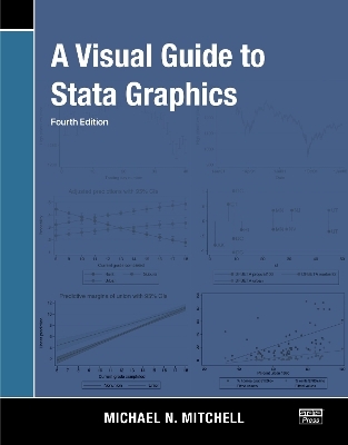
A Visual Guide to Stata Graphics
Stata Press (Verlag)
978-1-59718-365-9 (ISBN)
- Titel nicht im Sortiment
- Artikel merken
A complete guide to Stata's graph command
Exhaustive examples of customized graphs
Visual indexing of features-just look for a picture that matches what you want to do
This edition includes new discussions of color, Unicode characters, export formats, sizing of graph elements, and schemes. The section on colors has been greatly expanded to include over 50 examples that demonstrate how to modify colors, add transparency, and change intensity. In the discussion of text modifications, Mitchell now shows how to include Unicode characters such as Greek letters, symbols, and emojis. New examples have also been added that show how to change the size of graph elements such as text, markers, and line widths using both absolute units (points, inches, and centimeters) as well as relative units (line large or *2 for two times the original size). Finally, the look of graphs throughout the book has changed-most graphs are now created using a common updated scheme.
The book's visual style makes it easy to find exactly what you need. A color-coded, visual table of contents runs along the edge of every page and shows readers exactly where they are in the book. You can see the color-coded chapter tabs without opening the book, providing quick visual access to each chapter.
The heart of each chapter is a series of entries that are typically formatted three to a page. Each entry shows a graph command (with the emphasized portion of the command highlighted in red), the resulting graph, a description of what is being done, and the dataset used. Because every feature, option, and edit is demonstrated with a graph, you can often flip through a section of the book to find exactly the effect you are seeking.
The book begins with an introduction to Stata graphs that includes an overview of graphs types, schemes, and options and the process of building a graph. Then, it turns to detailed discussions of many graph types-scatterplots, regression fit plots, line plots, contour plots, bar graphs, box plots, and many others. Mitchell shows how to create each type of graph and how to use options to control the look of the graph. Because Stata's graph command will let you customize any aspect of the graph, Mitchell spends ample time showing you the most valuable options for obtaining the look you want. If you are in a hurry to discover one special option, you can skim the chapter until you see the effect you want and then glance at the command to see what is highlighted in red.
After focusing on specific types of graphs, Mitchell undertakes an in-depth presentation of the options available across almost all graph types. This includes options that add and change the look of titles, notes, and such; control the number of ticks on axes; control the content and appearance of the numbers and labels on axes; control legends; add and change the look of annotations; graph over subgroups; change the look of markers and their labels; size graphs and their elements; and more. To complete the graphical journey, Mitchell discusses and demonstrates the 12 styles that unite and control the appearance of the myriad graph objects. These styles are angles, colors, clock positions, compass directions, connecting points, line patterns, line widths, margins, marker sizes, orientations, marker symbols, and text sizes.
You won't want to overlook the appendix in this book. There Mitchell first gives a quick overview of the dozens of statistical graph commands that are not strictly the subject of the book. Even so, these commands use the graph command as an engine to draw their graphs; therefore, almost all that Mitchell has discussed applies to them. He also addresses combining graphs-showing you how to create complex and multipart images from previously created graphs. In a crucial section titled "Putting it all together", Mitchell shows us how to do just that. We learn more about overlaying twoway plots, and we learn how to combine data management and graphics to create plots such as bar charts of rates with capped confidence intervals. Mitchell concludes by warning us about mistakes that can be made when typing graph commands and how to correct them.
The fourth edition of A Visual Guide to Stata Graphics is a complete guide to Stata's graph command and the associated Graph Editor. Whether you want to tame the Stata graph command, quickly find out how to produce a graphical effect, or learn approaches that can be used to construct custom graphs, this is the book to read.
Michael N. Mitchell is a senior statistician working in the area of sleep research as well as working on prevention of child maltreatment with the Children's Data Network. He is the author of three other Stata Press books-Interpreting and Visualizing Regression Models Using Stata, Data Management Using Stata, and Stata for the Behavioral Sciences.
1 Introduction
1.1 Online supplements
1.2 Using this book
1.3 Types of Stata graphs
1.4 Schemes
1.4.1 Schemes included with Stata
1.4.2 Community-contributed schemes
1.4.3 Schemes included with this book
1.4.4 Setting schemes
1.5 Options
1.6 Building graphs
1.7 Point-and-click interface
2 Twoway graphs
2.1 Scatterplots
2.2 Regression fits and splines
2.3 Regression confidence interval fits
2.4 Line plots
2.5 Area plots
2.6 Bar plots
2.7 Range plots
2.8 Distribution plots
2.9 Contour plots
2.10 Options
2.11 Overlaying plots
3 Scatterplot matrix graphs
3.1 Marker options
3.2 Controlling axes
3.3 Matrix options
3.4 Graphing by groups
4 Bar graphs
4.1 Y variables
4.2 Graphing bars over groups
4.3 Options for controlling gaps between bars
4.4 Options for sorting bars
4.5 Controlling the categorical axis
4.6 Controlling the legend and labeling bars
4.7 Controlling the y axis
4.8 Changing the look of bars
4.9 Graphing by groups
5 Box plots
5.1 Specifying variables and groups
5.2 Options for controlling gaps between boxes
5.3 Options for sorting boxes
5.4 Controlling the categorical axis
5.5 Controlling the legend
5.6 Controlling the y axis
5.7 Changing the look of boxes
5.8 Graphing by groups
6 Dot plots
6.1 Specifying variables and groups
6.2 Options for controlling gaps between dots
6.3 Options for sorting dots
6.4 Controlling the categorical axis
6.5 Controlling the legend
6.6 Controlling the y axis
6.7 Changing the look of dot rulers
6.8 Graphing by groups
7 Pie charts
7.1 Types of pie charts
7.2 Sorting pie slices
7.3 Changing the look and color and exploding pie slices
7.4 Slice labels
7.5 Controlling the legend
7.6 Graphing by groups
8 Options available for most graphs
8.1 Changing the look of markers
8.2 Creating and controlling marker labels
8.3 Connecting points and markers
8.4 Setting and controlling axis titles
8.5 Setting and controlling axis labels
8.6 Controlling axis scales
8.7 Selecting an axis
8.8 Graphing by groups
8.9 Controlling the legend
8.10 Adding text to markers and positions
8.11 Options for text and textboxes
8.12 More options controlling the display of text
9 Standard options available for all graphs
9.1 Creating and controlling titles
9.2 Using schemes to control the look of graphs
9.2.1 Schemes included with Stata
9.2.2 Community-contributed schemes
Graph schemes sensitive to color vision deficiency
The 538 family of schemes
The lean family of schemes
9.2.3 Schemes included with this book
9.2.4 Example #1: An overlaid scatterplot with fit lines
9.2.5 Example #2: An overlaid scatterplot with fit lines and confidence region
Example #3: A bar chart
The grstyle way of customizing graphs
9.2.6 Customizing schemes
9.2.7 Using the set scheme command
9.3 Sizing graphs and their elements
9.3.1 Sizing/resizing graphs with absolutely sized versus relatively sized units
9.4 Changing the look of graph regions
10 Styles for changing the look of graphs
10.1 Angle
10.2 Color
10.2.1 Named colors
10.2.2 Color intensity
Increasing brightness
Decreasing brightness
The brightness spectrum
10.2.3 Color opacity
10.2.4 Overlapping colors
10.2.5 Specifying colors using RGB, CMYK, and HSV values
10.3 Clock position
10.4 Compass direction
10.5 Connecting points
10.6 Line patterns
10.7 Line width
10.8 Margin
10.9 Marker size
10.10 Orientation
10.11 Marker symbol
10.12 Text size
11 Appendix
11.1 Overview of statistical graph commands
11.2 Common options for statistical graphs
11.3 The marginsplot command
11.4 Saving, redisplaying, and combining graphs
11.5 Exporting graphs
11.6 More examples: Putting it all together
11.7 Common mistakes
| Erscheinungsdatum | 15.02.2022 |
|---|---|
| Zusatzinfo | over 1,200 illustrated colored examples |
| Verlagsort | College Station |
| Sprache | englisch |
| Gewicht | 1089 g |
| Themenwelt | Mathematik / Informatik ► Informatik |
| Mathematik / Informatik ► Mathematik ► Computerprogramme / Computeralgebra | |
| ISBN-10 | 1-59718-365-2 / 1597183652 |
| ISBN-13 | 978-1-59718-365-9 / 9781597183659 |
| Zustand | Neuware |
| Informationen gemäß Produktsicherheitsverordnung (GPSR) | |
| Haben Sie eine Frage zum Produkt? |
aus dem Bereich


