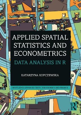
Applied Spatial Statistics and Econometrics
Routledge (Verlag)
978-0-367-47076-0 (ISBN)
This textbook is a comprehensive introduction to applied spatial data analysis using R. Each chapter walks the reader through a different method, explaining how to interpret the results and what conclusions can be drawn. The author team showcases key topics, including unsupervised learning, causal inference, spatial weight matrices, spatial econometrics, heterogeneity and bootstrapping. It is accompanied by a suite of data and R code on Github to help readers practise techniques via replication and exercises.
This text will be a valuable resource for advanced students of econometrics, spatial planning and regional science. It will also be suitable for researchers and data scientists working with spatial data.
Katarzyna Kopczewska is an associate professor at University of Warsaw, Faculty of Economic Sciences. As a quantitative economist, she deals with spatial modelling of geolocalised economic processes – location and co-location, agglomeration, concentration, diffusion, spatial interactions in relation to economic phenomena, companies and real estate but also regional policy or public-sector activities. She conducts methodological research on the implementation of data science methods for spatial analysis and combining them with classical spatial statistics and econometrics in R. She combines quantitative solutions with theory and problems of regional science and economic geography. She serves at the European Regional Science Association (ERSA).
Contents Introduction Statement by the American Statistical Association on statistical significance and p-value used in the book Acknowledgments Chapter 1: Basic operations in the R software (Mateusz Kopyt) 1.1 About the R software 1.2. The R software interface 1.2.1 R Commander 1.2.2. RStudio 1.3 Using help 1.4 Additional packages 1.5 R Language - basic features 1.6 Defining and loading data 1.7 Basic operations on objects 1.8 Basic statistics of the data set 1.9 Basic visualizations
1.9.1 Scatterplot and line chart 1.9.2 Column chart 1.9.3 Pie chart 1.9.4 Boxplot 1.10 Regression in examples Chapter 2: Spatial data, R classes and basic graphics (Katarzyna Kopczewska) 2.1 Loading and basic operations on spatial vector data 2.2. Creating, checking and converting spatial classes 2.3 Selected color palettes
2.4 Basic contour maps with a color layer Scheme 1 - with colorRampPalette() from the grDevices:: package Scheme 2 - with choropleth() from the GISTools:: package
Scheme 3 - with findInterval() from the base:: package Scheme 4 - with findColours() from the classInt:: package Scheme 5 - with spplot() from the sp:: package
2.5 Basic operations and graphs for point data Scheme 1 - with points() from the graphics:: package – locations only Scheme 2 - with spplot() from the sp:: package - locations and values Scheme 3 - with findInterval() from the base:: package - locations, values, different size of symbols 2.6 Basic operations on rasters 2.7 Basic operations on grids 2.8 Spatial geometries Chapter 3: Spatial data from the Web API (Mateusz Kopyt, Katarzyna Kopczewska) 3.1 What is the API? 3.2. Creating contextual maps with use of API 3.3 Ways to visualize spatial data - maps for point and regional data Scheme 1 - with bubbleMap() from the RgoogleMaps:: package Scheme 2 - with ggmap() from the ggmap:: package Scheme 3 - with PlotOnStaticMap() from the RgoogleMap:: package Scheme 4 - with RGoogleMaps:: GetMap() and conversion of staticMap into a raster 3.4 Spatial data in vector format - example of the OSM database 3.5 Access to non-spatial internet databases and resources via API - examples 3.6 Geo-coding of data Chapter 4: Spatial weight matrices, distance measurement, tessellation, spatial statistics (Katarzyna Kopczewska, Maria Kubara) 4.1. Introduction to spatial data analysis 4.2 Spatial weights matrix 4.2.1 General framework for creating spatial weights matrices 4.2.2 Selection of a neighborhood matrix 4.2.3 Neighborhood matrices according to the contiguity criterion 4.2.4 Matrix of k nearest neighbors (knn) 4.2.5 Matrix based on distance criterion (neighbours in a radius of d km) 4.2.6 Inverse distance matrix 4.2.7 Summarizing and editing of spatial weights matrix 4.2.8 Spatial lags and higher order neighborhood 4.2.9 Creating weights matrix based on group membership 4.3 Distance measurement and spatial aggregation 4.4 Tessellation 4.5 Spatial statistics 4.5.1 Global statistics 4.5.1.1 Global Moran I statistics 4.5.1.2 Global Geary C statistics 4.5.1.3 Join-count statistics 4.5.2. Local spatial autocorrelation statistics 4.5.2.1 Local Moran I statistics (LISA)
4.5.2.2 Local Geary C statistics 4.5.2.3 Local Getis-Ord Gi statistics 4.5.2.4. Local spatial heteroscedasticity (LOSH) 4.6 Spatial cross-correlations for two variables 4.7 Correlogram Chapter 5: Applied spatial econometrics (Katarzyna Kopczewska) 5.1 Value added from spatial modelling and classes of models 5.2 Basic cross-sectional models 5.2.1 Estimation 5.2.2 Quality assessment of spatial models 5.2.2.1 Information criteria and pseudo R2 in assessing model fit 5.2.2.2 Test for heteroskedasticity of model residuals 5.2.2.3 Residual autocorrelation tests 5.2.2.4 LM tests for model type selection 5.2.2.5 LR and Wald tests for model restrictions
5.2.3 Selection of spatial weight matrix and modelling of diffusion strength 5.2.4 Forecasts in spatial models 5.2.5 Causality 5.3 Selected specifications of cross-sectional spatial models 5.3.1 Uni-directional spatial interaction models 5.3.2 Cumulative models 5.3.3 Bootstrapped models for big data 5.3.4 Models for grid data
5.4 Spatial panel models Chapter 6: Geographically Weighted Regression - modelling spatial heterogeneity (Piotr Ćwiakowski) 6.1 Geographically weighted regression
6.2 Basic estimation of GWR model 6.2.1 Estimation of the reference OLS model 6.2.2 Choosing the optimal bandwidth for a dataset 6.2.3 Local geographically weighted statistics 6.2.4 Geographically weighted regression estimation 6.2.5 Basic diagnostic tests of the GWR model 6.2.6 Testing the significance of parameters in GWR 6.2.7 Selection of the optimal functional form of the model 6.2.8 GWR with heteroskedastic random error 6.3 The problem of collinearity in GWR models 6.3.1 Diagnosing collinearity in GWR 6.4. Mixed GWR 6.5. Robust regression in the GWR model 6.6. Geographically and Temporally Weighted Regression (GTWR) Chapter 7: Unattended spatial learning (Katarzyna Kopczewska) 7.1 Clustering of spatial points with k-means, PAM and CLARA algorithms 7.2 Clustering with the DBSCAN algorithm 7.3 Spatial Principal Component Analysis 7.4 Spatial Drift 7.5 Spatial hierarchical clustering 7.6 Spatial oblique decision tree Chapter 8: Spatial point pattern analysis and spatial interpolation (Kateryna Zabarina) 8.1. Introduction and main definitions 8.1.1. Dataset 8.1.2. Creation of window and point pattern 8.1.3. Marks 8.1.4. Covariates 8.1.5. Duplicated points 8.1.6. Projection and rescaling 8.2. Intensity-based analysis of unmarked point pattern 8.2.1. Quadrat test 8.2.2. Tests with spatial covariates 8.3. Distance-based analysis of the unmarked point pattern 8.3.1. Distance-based measures 8.3.1.1. Ripley’s K function 8.3.1.2. F function 8.3.1.3. G function 8.3.1.4. J function 8.3.1.5. Distance-based CSR tests 8.3.2. Monte-Carlo tests 8.3.3. Envelopes 8.3.4. Non-graphical tests 8.4. Selection and estimation of a proper model for unmarked point pattern 8.4.1. Theoretical note 8.4.2. Choice of parameters 8.4.3. Estimation and results 8.4.4. Conclusions 8.5. Intensity-based analysis of marked point pattern 8.5.1. Segregation test 8.6. Correlation and spacing analysis of the marked point pattern 8.6.1. Analysis under assumption of stationarity 8.6.1.1. K function variations for multitype pattern 8.6.1.2. Mark connection function 8.6.1.3. Analysis of within and between types of dependence
8.6.1.4. Randomisation test of components’ independence 8.6.2. Analysis under assumption of non-stationarity 8.6.2.1. Inhomogeneous K function variations for multitype pattern 8.7. Selection and estimation of a proper model for unmarked point pattern 8.7.1. Theoretical note 8.7.2. Choice of optimal radius 8.7.3. Within-industry interaction radius 8.7.4. Between-industry interaction radius 8.7.5. Estimation and results 8.7.6. Model with no between-industry interaction 8.7.7. Model with all possible interactions 8.8. Spatial interpolation methods - kriging 8.8.1. Basic definitions 8.8.2. Description of chosen kriging methods 8.8.3. Data preparation for the study 8.8.4. Estimation and discussion Chapter 9: Spatial Sampling and Bootstrap (Katarzyna Kopczewska, Piotr Ćwiakowski) 9.1 Spatial point data - object classes and spatial aggregation 9.2 Spatial sampling - randomization / generation of new points on the surface 9.3 Spatial sampling - sampling of sub-samples from existing points 9.3.1 Simple sampling 9.3.2 The options of the sperrorest:: package 9.3.3 Sampling points from areas determined by the k-means algorithm - block bootstrap
9.3.4 Sampling points from moving blocks (moving block bootstrap, MBB) 9.4. The use of spatial sampling and bootstrap in cross-validation of models Chapter 10: Spatial Big Data (Piotr Wójcik) 10.1. Examples of big data usage 10.2. Spatial big data 10.2.1. Spatial data types 10.2.2. Challenges related to the use of spatial Big Data
10.2.2.1. Processing of large data sets 10.2.2.2. Mapping and reduction 10.2.2.3. Spatial data indexing 10.3. The sf:: package - simple features 10.3.1 sf class – a special data frame 10.3.2 Data with POLYGON geometry 10.3.3 Data with POINT geometry 10.3.4 Visualization using the ggplot2:: package 10.3.5 Selected functions for spatial analysis 10.4. Using the dplyr:: package functions 10.5. Example analysis of large raster data 10.5.1. Measurement of economic inequalities from space
10.5.2. Analysis using the raster:: package functions 10.5.3 Other functions of the raster:: package 10.5.4 Potential alternative – stars:: package Chapter 11: Spatial unsupervised learning – applications of market basket analysis in geomarketing (Alessandro Festi) 11.1 Introduction to market basket analysis 11.2 Data needed in spatial market basket analysis 11.3 Simulation of data 11.4 The market basket analysis technique applied to geolocation data 11.5 Spatial association rules
11.6 Applications to geomarketing 11.6.1 Finding the best location for a business 11.6.2 Targeting 11.6.3 Discovery of competitors 11.7 Conclusions and further approaches Appendix 1: Data used in the examples A1. Data set No. 1 / dataset1 / - poviat panel data with many variables A2. Dataset no 2 /dataset2/ – geo-located point data A3. Dataset no 3 /dataset3/ – monthly unemployment rate in poviats (NTS4) A4. Dataset no 4 /dataset4/ - grid data for population A5. Shapefiles of countour maps – for poviats (NTS4), regions (NTS2), country (NTS0) and registration areas A6. Raster data on night light intensity on Earth in 2013 A7. Population in cities in Poland Appendix 2: Links between packages Appendix 3: Spatial data sets in R packages References Index of terms Index of R packages Index of R commands
| Erscheinungsdatum | 15.01.2021 |
|---|---|
| Reihe/Serie | Routledge Advanced Texts in Economics and Finance |
| Zusatzinfo | 10 Tables, black and white; 200 Illustrations, black and white |
| Verlagsort | London |
| Sprache | englisch |
| Maße | 210 x 280 mm |
| Gewicht | 2000 g |
| Themenwelt | Mathematik / Informatik ► Informatik ► Theorie / Studium |
| Naturwissenschaften ► Biologie ► Ökologie / Naturschutz | |
| Naturwissenschaften ► Geowissenschaften ► Geografie / Kartografie | |
| Wirtschaft ► Volkswirtschaftslehre ► Ökonometrie | |
| ISBN-10 | 0-367-47076-4 / 0367470764 |
| ISBN-13 | 978-0-367-47076-0 / 9780367470760 |
| Zustand | Neuware |
| Informationen gemäß Produktsicherheitsverordnung (GPSR) | |
| Haben Sie eine Frage zum Produkt? |
aus dem Bereich


