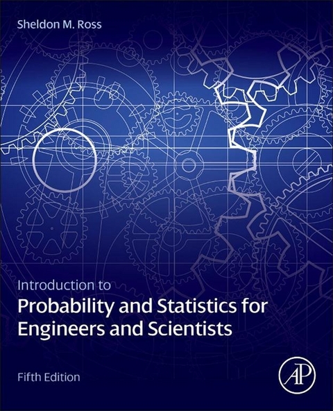
Introduction to Probability and Statistics for Engineers and Scientists (eBook)

Sheldon M. Ross (Autor)

eBook Download: PDF | EPUB

2014 | 5. Auflage
686 Seiten
Elsevier Science (Verlag)
978-0-12-394842-7 (ISBN)

Infos

Introduction to Probability and Statistics for Engineers and Scientists, Fifth Edition is a proven text reference that provides a superior introduction to applied probability and statistics for engineering or science majors. The book lays emphasis in the manner in which probability yields insight into statistical problems, ultimately resulting in an intuitive understanding of the statistical procedures most often used by practicing engineers and scientists. Real data from actual studies across life science, engineering, computing and business are incorporated in a wide variety of exercises and examples throughout the text. These examples and exercises are combined with updated problem sets and applications to connect probability theory to everyday statistical problems and situations. The book also contains end of chapter review material that highlights key ideas as well as the risks associated with practical application of the material. Furthermore, there are new additions to proofs in the estimation section as well as new coverage of Pareto and lognormal distributions, prediction intervals, use of dummy variables in multiple regression models, and testing equality of multiple population distributions. This text is intended for upper level undergraduate and graduate students taking a course in probability and statistics for science or engineering, and for scientists, engineers, and other professionals seeking a reference of foundational content and application to these fields. - Clear exposition by a renowned expert author - Real data examples that use significant real data from actual studies across life science, engineering, computing and business - End of Chapter review material that emphasizes key ideas as well as the risks associated with practical application of the material - 25% New Updated problem sets and applications, that demonstrate updated applications to engineering as well as biological, physical and computer science - New additions to proofs in the estimation section - New coverage of Pareto and lognormal distributions, prediction intervals, use of dummy variables in multiple regression models, and testing equality of multiple population distributions.

Dr. Sheldon M. Ross is a professor in the Department of Industrial and Systems Engineering at the University of Southern California. He received his PhD in statistics at Stanford University in 1968. He has published many technical articles and textbooks in the areas of statistics and applied probability. Among his texts are A First Course in Probability, Introduction to Probability Models, Stochastic Processes, and Introductory Statistics. Professor Ross is the founding and continuing editor of the journal Probability in the Engineering and Informational Sciences. He is a Fellow of the Institute of Mathematical Statistics, a Fellow of INFORMS, and a recipient of the Humboldt US Senior Scientist Award.

Textauszug

Setting equal to 0 gives

i=1nxi+∑i=1nwi=2nμ1+nμ2∑i=1nyi+∑i=1nwi=nμ1+2nμ2

yielding ^1=2Σxi+Σwi−Σyi3n,μ^2=2Σyi+Σwi−Σxi3n

6. The average of the distances is i50.456, and that of the angles is 40.27. Using these estimates the length of the tower, call it T, is estimated as follows:

=Xtanθ≈127.461

7. With Y = log(X), then X = eY. Because Y is normal with parameters μ and σ2

X=EeY=eμ+σ2/2EX2=Ee2Y=e2μ+2σ2

giving that

X=e2μ+2σ2−e2μ+σ2

(c) Taking the sample mean and variance of the logs of the data, yields the estimates that ^=3.7867,σ^2=.0647. Hence, the estimate of E[X] is μ^+σ^2/2=45.561.

8. ¯=3.1502

(a). ±1.96.1/5=3.06253.2379

(b). ±12.58.1/5=3.03483.2656

9. ¯=11.48

(a) ±1.96.08/10=11.48±.0496

(b) ∞,11.48±1.645.08/10=−∞,11.5216

(c) −1.645.08/10,∞=11.4384∞

10. 74.6 ± 1.645(11.3)/9 = 74.6 ± 2.065 = (72.535, 76.665)

11. 

(a) Normal with mean 0 and variance 1 + 1/n

(b) With probability ,−1.64<Xn+1−X¯n/1+1/n<1.64. Therefore, with 90 percent confidence, n+1∈X¯n±1.641+1/n.

12. nμ−X¯/σ<zα=1−α and so μ<X¯+zασ/n=1−α

13. ±z.0050.2/20or1.04841.3152

14. ±t.005,19.2/20or1.07201.3280

15. ±t.01,19.2/20=1.31359

16. The size of the confidence interval will be tα/2,n−1Sn/n≃2za/2σ/n for n large. First take a subsample of size 30 and use its sample standard deviation, call it σe, to estimate σ. Now choose the total sample size n (= 30 + additional sample size) to be such that zα/2σe/n≤A. The final confidence interval should now use all n values.

17. Run program 7-3-1. The 95 percent interval is (331.0572, 336.9345), whereas the 99 percent interval is (330.0082, 337.9836).

18. 

(a) (128.14, 138.30)

(b) (−∞, 129.03)

(c) (137.41, ∞)

19. Using that t.05,8 = 1.860, shows that, with 95 percent confidence, the mean price is above

,000−1.86012000/3=129,440114,560

20. 2, 200 ± 1.753(800)/4 = 2, 200 ± 350.6

21. Using that t.025,99 = 1.985, show that, with 95 percent confidence, the mean score is in the interval 320 ± 1.985(16)/10 = 320 ± 3.176

22. ±2.09415.4/20,330.2±2.86115.4/20 where the preceding used that t.025,19 = 2.0 94, t.005,19 = 2.861.

23. ±1.968840/300, since t.025,299 = 1.968

24. ±1.284840/300, since t.10,299 = 1.284

26. (a) (2013.9, 2111.6), (b) (1996.0,2129.5) (c) 2022.4

27. (93.94, 103.40)

28. (.529, .571)

29. E[N] = e

30. (10.08, 13.05)

31. (85, 442.15, 95, 457.85)

32. n+1−X¯n is normal with mean 0 and variance σ2 + σ 2/n. Hence, [Xn+1−X¯n)2=σ21+1/n.

33. (3.382, 6.068)

34. 3.007

36. 32.23, (12.3, 153.83, 167.2), 69.6

37. (.00206, .00529)

38. 3S12+13S22=4

39. .008

40. Use the fact that nT2/σ2 is chi-square with n degrees of freedom, where T2 ∑ i = 1n(Xi − μ)2/n. This gives that X¯−μ/T is a t-random variable with n degrees of freedom. The confidence interval is ¯−tα2,nT/n,X¯+tα2,nT/n. The additional degree of freedom is like having an extra observation.

41. (− 22.84, 478.24), (20.91, ∞), (−∞, 434.49)

42. (− 11.18, − 8.82)

43. (− 11.12, − 8.88)

44. (− 74.97, 41.97)

45. Using that

y2/σ22Sx2/σ12

has an F-distribution with parameters m − 1 and n − 1 gives the following 100(1 – α) percent confidence interval for σ12/σ22

1−α/2,m−1,n−1Sx2/Sy2,Fα/2,m−1,n−1Sx2/Sy2

47. 

(a) .396 ± .024 [.372, .42]

(b) .389 ± .037 [.352, .426]

48. .17 ± .018, .107 ± .015

49. .5106 ± .010, .5106 ± .013

50. 1692

51. no

52. 2401

53. .00579×61/140/140=.108

54. ±17×.83/100=.096,.244,.073,.267

55. .67 An additional sample of size 2024 is needed.

57. (21.1, 74.2)

58. Since

{2∑Xi/θ>χ1−α,2n2}=1−α

it follows that the lower confidence interval is given by

<2∑Xi/χ1−α,2n2

Similarly, a 100(1 – α) percent upper confidence interval for θ is

<2∑Xi/χα,2n2

60. Since Var[(n − 1)Sx2/σ2] = 2(n − 1) it follows that Var(Sx2) = 2σ4/(n − 1) and similarly Var(Sy2) = 2σ4/(n − 1). Hence, using Example 5.5b which shows that the best weights are inversely proportional to the variances, it follows that the pooled estimator is best.

61. As the risk of d1 is 6 whereas that of d2 is also 6 they are equally good.

62. Since the number of accidents over the next 10 days is Poisson with mean 10 k it follows that P{83|λ} = e− 10λ(10λ)83/83!. Hence,

λ|83=P83|λe−λ∫P83|λe−λdλ=cλ83e−11λ

where c does not depend on λ. Since this is the gamma density with parameters 84.11 it has mean 84/11 = 7.64 which is thus the Bayes estimate. The maximum likelihood estimate is 8.3. (The reason that the Bayes estimate is smaller is that it incorporates our initial belief that λ can be thought of as being the value of an exponential random variable with mean 1.)

63. λ|x1…xn=fx1…xn|λgλ/c=cλne−λΣxie−λλ2=cλn+2e−λ1+Σxi
where c × p(x1 … xn) does not depend on λ. Thus we see that the posterior distribution of λ is the gamma distribution with parameters n + 3.1 + Σxi: and so the Bayes estimate is (n + 3)/(1 + Σxi), the mean of the posterior distribution. In our problem this yields the estimate 23/93.

64. The posterior density of p is, from Equation (5.5.2) f (p|data) = 11!pi(1 − p)10 − i/1!(10 - i)! where i is the number of defectives in the sample of 10. In all cases the desired probability is obtained by integrating this density from p equal 0 to p equal .2. This has to be done numerically as the above does not have a closed form integral.

65 The posterior distribution is normal with mean 80/89(182) + 9/89(200) = 183.82 and...

Produkt-Details

• Erscheint lt. Verlag: 14.8.2014
• Sprache: englisch
• Themenwelt: Mathematik / Informatik ► Mathematik ► Angewandte Mathematik
• Themenwelt: Mathematik / Informatik ► Mathematik ► Statistik
• Themenwelt: Mathematik / Informatik ► Mathematik ► Wahrscheinlichkeit / Kombinatorik
• Themenwelt: Technik
• ISBN-10: 0-12-394842-8 / 0123948428
• ISBN-13: 978-0-12-394842-7 / 9780123948427